Training an autoencoder

In this section, we'll train a type of neural network called an autoencoder as an alternative to other dimensionality reduction algorithms such as tSNE or UMAP. In the cluster analysis section, we'll create embeddings to our datasets from the deep learning model we train in this section.

What is an autoencoder?

An autoencoder is a type of generative neural network. Generative in this context means it will create an artificial expression profile mimicking our real data. However we are not actually interested in the generated data but rather one of the internal layers called the latent dimension. This can represent our data in a lower dimensionality in a similar way that PCA or UMAP can. Although it should be noted that neural networks can learn non-linear characteristics of our data due to something called activation functions in each layer. Without activation functions, neural networks would only have linear transformations stacked on top of the other at each layer and therefore couldn't detect complex non-linearities in our dataset. Detecting non-linearities substantially reduces the reconstruction loss when generating our synthetic cell transcriptome data. To summarize:

• We pass our data through the neural network. In the first pass our network weights and biases (see below) are initialized over a Gaussian distribution
• We calculate a reconstruction loss using a loss function. In our case the loss function is defined as being the difference between the original cell transcriptomes and the predicted cell transcriptomes.
• We now try to reduce the reconstruction loss by adjusting our weights and biases slightly in a process called backpropogation. This can be done by calculating the partial derivative (a multivariate gradient function - multivariate because we have weight, bias and input params to consider) on each function between layers. This lets us know in which direction to adjust our network parameters.
• When we've reached a satisfactory value for our loss function, or reached the end of our training epochs, we can finally extract the latent dimension in the neural network. In the diagram below we have 3 neurons which would represent the x, y and z axis. In practice this could be much larger, for example 100 neurons, so further dimensionality reduction would be required.

Below shows a simplified version of an autoencoder, notice how the encoder and decoder are mirror images of each other:

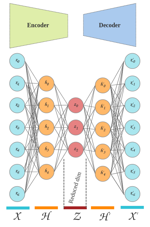
Not shown: weights and activation functions

Layers

• X: Input layer, each neuron will receive as input the gene expression values in each cell's transcriptome.
• H: Hidden layer(s), at least one hidden layer is required in our network.
• Z: Latent layer, This represents our lowest dimensionality of the data. Once the training is finished, we will extract this layer for visualizing clusters.
• H': The reverse of the first hidden layer from the encoder.
• X': This is the output layer (also the reverse of the first input layer). Notice how this is the same shape as our inputs? This is because it is actually an artificially generated expression profile of our original data.

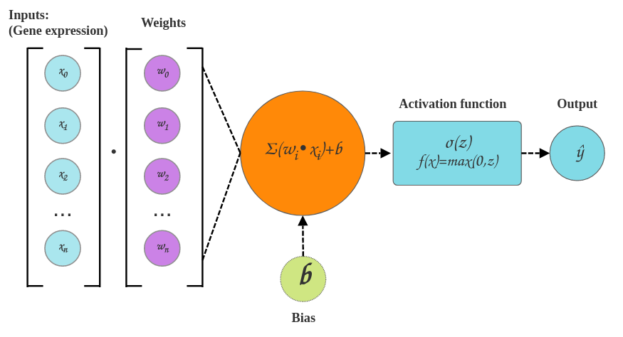
Single perceptron

Training an autoencoder in Nuwa

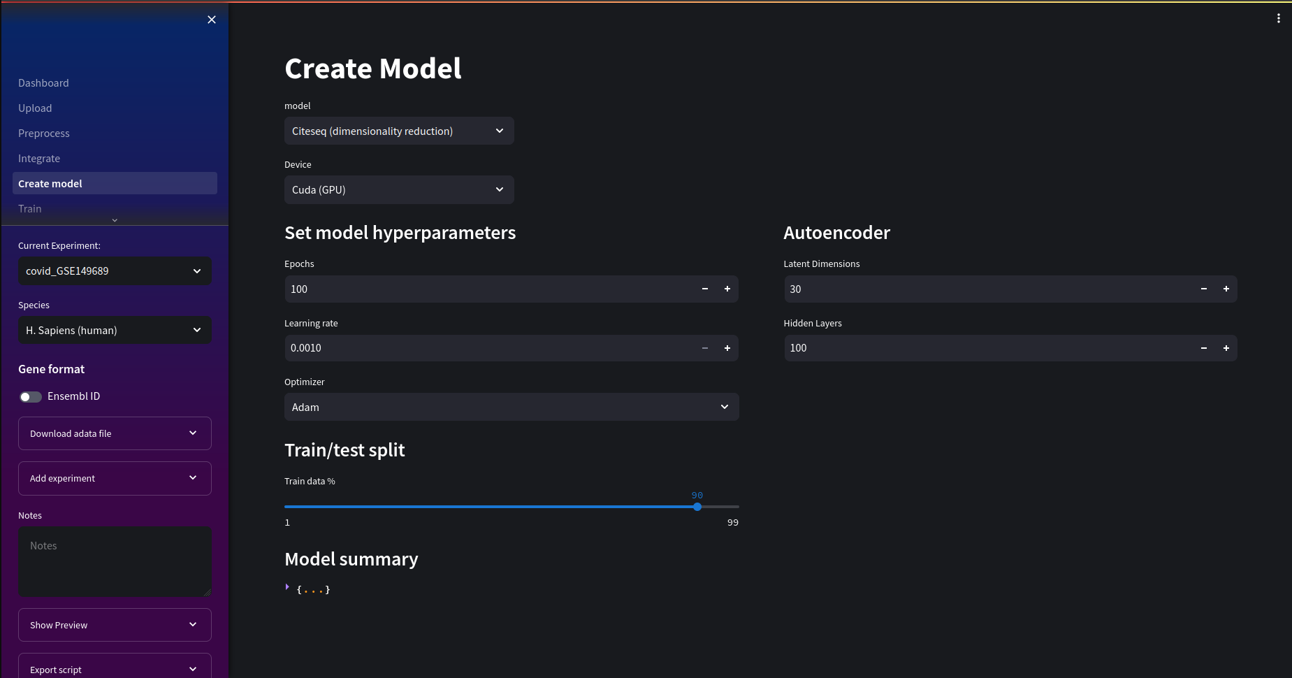
In the create model page, we will use the Citeseq model. We can adjust hyperparamers to suit our training needs. This includes things like epoch number, learning rate optimizer. For this tutorial we'll use the default values.

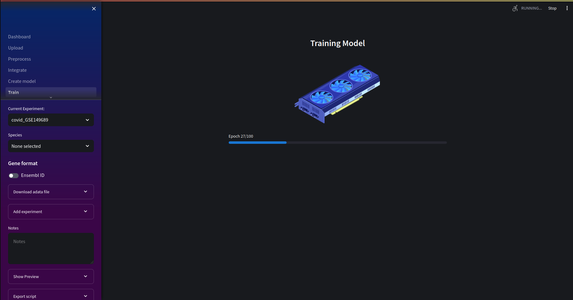
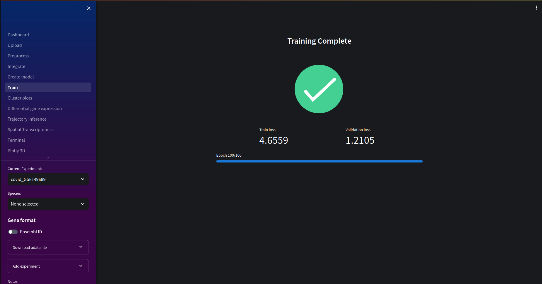
Next, we can go to the training page. If you are training on cuda device you'll notice a significant reduction in training time. If not, the animation will be different to the one below and will take longer to train.

Once our training is complete we can see the final training and validation loss. In the next section, we'll be able to see the convergence of training and validation losses over epochs. If the loss value is too high, or the embeddings in the cluster plots seem to yield less than useful insights, you may wish to retrain your model with different hyperparameters.

For a more in-depth article about autoencoders try this one by v7 labs.